Modeling the global geomagnetic field
Advanced Earth electromagnetism Homework-3
Methods and data
According to the Gauss Theory of geomagnetism, we can use the spherical harmonic analysis to describe the earth’s main magnetic field. Suppose the magnetic potential of the geomagnetic field obeys Laplace’s equation at the surface of the Earth as well as outside of the Earth, the model can be written as:
The only uncertainty in the formula is $g_n^m$ and $h_n^m$, which called Gauss Coefficient, and when we have the model and the data, we can get the parameters value by inversion methods. The problem becomes solving the following system of linear algebraic equations (the observations are taken at a spherical surface of the Earth’s mean radius, $r=a$ ):
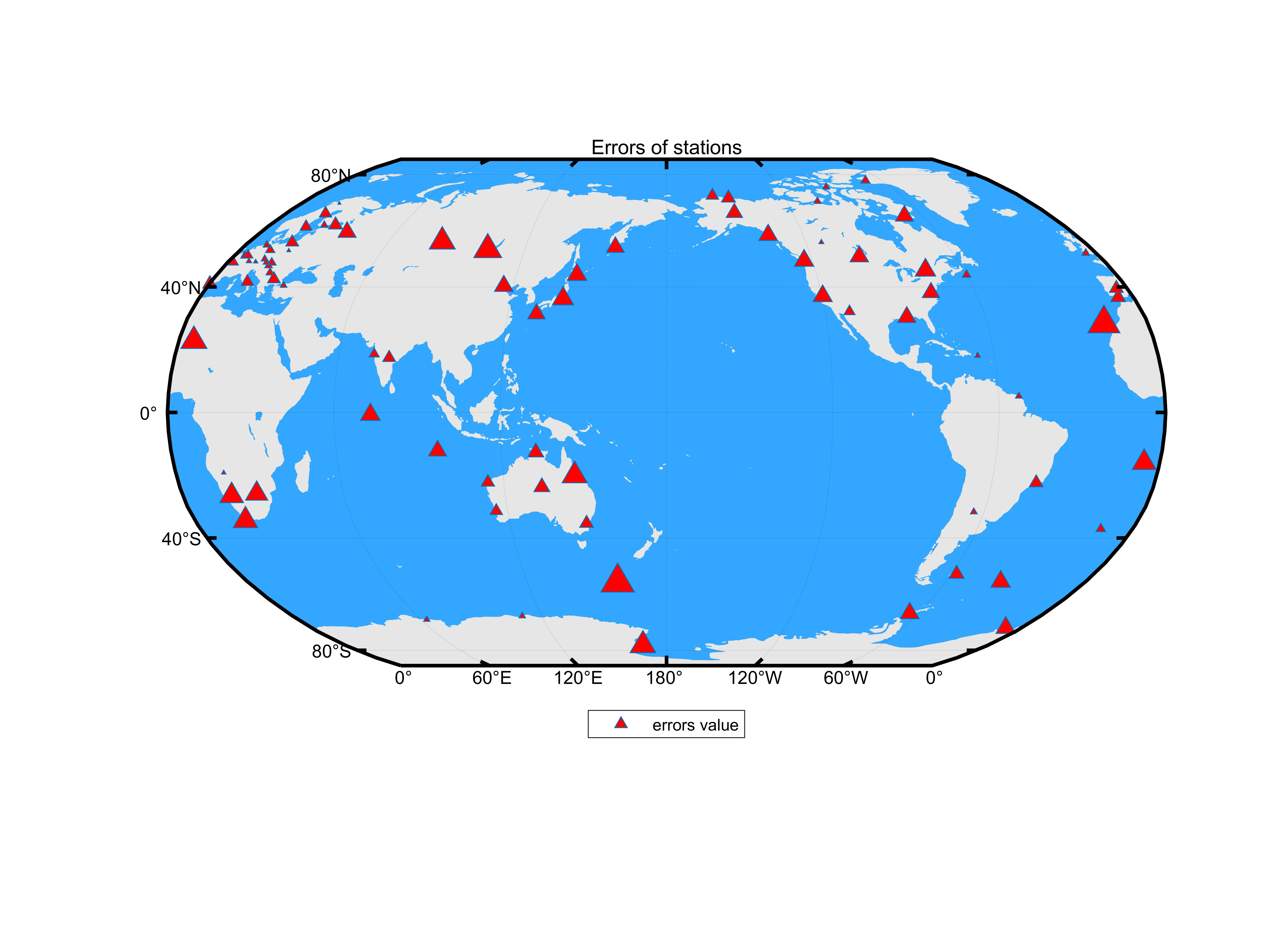
The data in $\mathbf{d}$ are download from INTERMAGNET, the website is https://www.intermagnet.org/data-donnee/download-eng.php. I selected the definitive minute data on 2020-03-05 (Table 1), all available observation stations are included, Figure 1 is a map showing the observatories I used. the 24-hour data of each station are averaged to obtain the observed values of the day, after eliminating the outliers. I wrote a MATLAB script to implement the above process, and built a model up to spherical harmonic degree 4.
Tab 1. A table of data
| Index | Name | Latitude | Longitude | X | Y | Z | Date | Index | Name | Latitude | Longitude | X | Y | Z | Date |
|---|---|---|---|---|---|---|---|---|---|---|---|---|---|---|---|
| 1 | abg | 18.62 | 72.87 | 38255.32861 | 290.4123611 | 20393.29507 | 20200305 | 42 | kdu | -12.686 | 132.472 | 35457.00736 | 1754.704167 | -29582.17056 | 20200305 |
| 2 | abk | 68.358 | 18.823 | 11263.29438 | 1862.256042 | 52149.73104 | 20200305 | 43 | kep | -54.282 | 323.507 | 15328.23479 | -1902.493542 | -22927.075 | 20200305 |
| 3 | aia | -65.25 | 295.73 | 19743.62451 | 5529.188194 | -31781.59625 | 20200305 | 44 | kmh | -26.541 | 18.11 | 10625.24368 | -3290.684375 | -24317.20576 | 20200305 |
| 4 | asp | -23.761 | 133.883 | 30118.9534 | 2384.582361 | -43746.81958 | 20200305 | 45 | kny | 31.424 | 130.88 | 32523.31208 | -3937.392708 | 33352.49993 | 20200305 |
| 5 | bdv | 49.08 | 14.015 | 20408.24278 | 1476.498472 | 44384.11257 | 20200305 | 46 | kou | 5.21 | 307.269 | 26566.90834 | -8649.159903 | 6534.03419 | 20200305 |
| 6 | bel | 51.836 | 20.789 | 18910.50938 | 2155.445069 | 46753.62417 | 20200305 | 47 | lrm | -22.222 | 114.101 | 30377.57938 | 113.0718056 | -43262.77563 | 20200305 |
| 7 | bfo | 48.331 | 8.325 | 21000.85431 | 971.8170139 | 43518.68674 | 20200305 | 48 | lyc | 64.612 | 18.748 | 12954.21903 | 1788.108194 | 50824.92569 | 20200305 |
| 8 | bmt | 40.3 | 116.2 | 27901.35056 | -4109.268472 | 47580.71354 | 20200305 | 49 | mab | 50.298 | 5.683 | 20026.52454 | 676.6008535 | 44643.7574 | 20200305 |
| 9 | box | 58.07 | 38.23 | 15149.76771 | 3423.754653 | 50605.48924 | 20200305 | 50 | maw | -67.6 | 62.88 | 6637.389861 | -17331.47576 | -45610.43313 | 20200305 |
| 10 | brd | 49.87 | 260.026 | 15215.71021 | 1349.588194 | 54525.18188 | 20200305 | 51 | mcq | -54.5 | 158.95 | 10702.30986 | 6865.926042 | -62729.04792 | 20200305 |
| 11 | brw | 71.32 | 203.38 | 8896.940417 | 2040.051944 | 56567.42097 | 20200305 | 52 | mea | 54.616 | 246.653 | 13676.0725 | 3502.193194 | 55141.94083 | 20200305 |
| 12 | bsl | 30.35 | 270.364 | 23897.89611 | -534.3659028 | 40619.165 | 20200305 | 53 | mmb | 43.91 | 144.189 | 25860.92479 | -4160.602986 | 42601.24806 | 20200305 |
| 13 | cbb | 69.123 | 254.969 | 5052.641181 | 515.9493056 | 58112.67063 | 20200305 | 54 | ngk | 52.072 | 12.675 | 18870.10889 | 1331.096806 | 45797.97604 | 20200305 |
| 14 | cki | -12.187 | 96.834 | 34897.57944 | -1267.207778 | -32411.88188 | 20200305 | 55 | nur | 60.508 | 24.655 | 14746.53667 | 2287.914931 | 50328.62708 | 20200305 |
| 15 | clf | 48.025 | 2.26 | 21268.24681 | 374.1634028 | 43038.32201 | 20200305 | 56 | nvs | 54.85 | 83.23 | 15977.18264 | 2267.85125 | 57794.77472 | 20200305 |
| 16 | cmo | 64.871 | 212.139 | 12071.0441 | 3662.327361 | 55060.79042 | 20200305 | 57 | ott | 45.403 | 284.448 | 18006.06139 | -4293.210347 | 50757.78646 | 20200305 |
| 17 | cnb | -35.314 | 149.363 | 23121.84965 | 5192.365069 | -52948.43965 | 20200305 | 58 | pag | 42.515 | 24.177 | 23724.57785 | 2052.341181 | 41095.60694 | 20200305 |
| 18 | cpl | 17.293 | 78.92 | 39453.13201 | -510.5802778 | 17435.07875 | 20200305 | 59 | pet | 52.971 | 158.248 | 21521.23347 | -2453.807986 | 47410.99722 | 20200305 |
| 19 | csy | -66.28 | 110.53 | -1183.919167 | -8905.680139 | -63455.59493 | 20200305 | 60 | pil | -31.667 | 296.119 | 18525.13889 | -1971.772847 | -12926.00313 | 20200305 |
| 20 | cta | -20.09 | 146.264 | 31415.04941 | 4032.899791 | -37523.00592 | 20200305 | 61 | pst | -51.704 | 302.107 | 17998.51828 | 816.7563025 | -21589.41492 | 20200305 |
| 21 | dou | 50.1 | 4.599 | 20166.69694 | 564.5751389 | 44377.19028 | 20200305 | 62 | res | 74.69 | 265.105 | 2821.225278 | -966.5449306 | 57412.04722 | 20200305 |
| 22 | dur | 41.65 | 14.467 | 24664.39583 | 1661.169444 | 39635.57229 | 20200305 | 63 | sba | -77.85 | 166.762 | -10322.08271 | 5515.313542 | -65094.66458 | 20200305 |
| 23 | ebr | 40.957 | 0.333 | 25322.75201 | 348.5455556 | 37632.16313 | 20200305 | 64 | sbl | 43.932 | 299.991 | 20099.86778 | -6159.527222 | 45830.59819 | 20200305 |
| 24 | frd | 38.201 | 282.63 | 21211.1253 | -3948.038707 | 45969.93919 | 20200305 | 65 | sfs | 36.667 | 354.055 | 27692.98333 | -437.525625 | 33061.71813 | 20200305 |
| 25 | frn | 37.091 | 240.281 | 22610.76882 | 5106.934306 | 41905.74014 | 20200305 | 66 | she | -15.961 | 354.253 | 16010.89917 | -3784.684444 | -25849.75875 | 20200305 |
| 26 | fur | 48.165 | 11.277 | 20993.37243 | 1266.938681 | 43689.14313 | 20200305 | 67 | sit | 57.058 | 224.675 | 15003.98639 | 5020.095972 | 52959.09139 | 20200305 |
| 27 | gan | -0.695 | 73.154 | 38064.10701 | -2720.955278 | -12852.37549 | 20200305 | 68 | sjg | 18.111 | 293.85 | 26371.23667 | -6125.861667 | 24778.29694 | 20200305 |
| 28 | gck | 44.63 | 20.77 | 22705.50861 | 1968.7925 | 42322.95653 | 20200305 | 69 | spg | 60.542 | 29.716 | 14451.77243 | 2766.171111 | 50554.4159 | 20200305 |
| 29 | gng | -31.356 | 115.715 | 24154.41201 | -695.7534028 | -52657.5475 | 20200305 | 70 | spt | 39.547 | 355.651 | 26157.41243 | -212.2654861 | 35974.31007 | 20200305 |
| 30 | gui | 28.321 | 343.559 | 27788.94125 | -3297.265486 | 22532.55771 | 20200305 | 71 | tam | 22.792 | 5.53 | 33853.35556 | 317.1153472 | 17125.37632 | 20200305 |
| 31 | had | 50.995 | 355.516 | 19815.59375 | -487.1833333 | 44458.94479 | 20200305 | 72 | tdc | -37.067 | 347.684 | 9158.353472 | -3520.939514 | -22389.23111 | 20200305 |
| 32 | hbk | -25.883 | 27.707 | 12484.80071 | -4183.221111 | -24963.03222 | 20200305 | 73 | thl | 77.47 | 290.77 | 3048.201319 | -2836.9075 | 56138.82771 | 20200305 |
| 33 | her | -34.425 | 19.225 | 9607.833819 | -4713.809861 | -22995.42292 | 20200305 | 74 | thy | 46.9 | 17.893 | 21518.14722 | 1798.217431 | 43480.7241 | 20200305 |
| 34 | hlp | 54.603 | 18.811 | 17482.39139 | 1693.542639 | 47405.90799 | 20200305 | 75 | tsu | -19.202 | 17.584 | 14031.38007 | -2157.920833 | -25488.01035 | 20200305 |
| 35 | hrb | 47.875 | 18.19 | 20998.77708 | 1814.178403 | 44071.71535 | 20200305 | 76 | tuc | 32.174 | 249.266 | 23874.2234 | 3757.009861 | 40291.74611 | 20200305 |
| 36 | hyb | 17.42 | 78.55 | 39586.70764 | -409.4116667 | 18254.32278 | 20200305 | 77 | ups | 59.903 | 17.353 | 15093.9141 | 1687.224931 | 49301.94847 | 20200305 |
| 37 | iqa | 63.756 | 291.49 | 8624.755702 | -3943.983658 | 56107.03804 | 20200305 | 78 | vic | 48.517 | 236.583 | 18091.75582 | 5186.817181 | 49871.91367 | 20200305 |
| 38 | irt | 52.17 | 104.45 | 18339.39819 | -1321.375208 | 57631.08368 | 20200305 | 79 | vna | -70.683 | 351.718 | 18066.2466 | -4484.883403 | -33255.14722 | 20200305 |
| 39 | izn | 40.5 | 29.72 | 25075.98528 | 2459.532708 | 40544.37868 | 20200305 | 80 | vss | -22.4 | 316.35 | 16425.94375 | -6916.265278 | -14993.05438 | 20200305 |
| 40 | jco | 70.356 | 211.201 | 8698.91 | 2596.038472 | 56590.54382 | 20200305 | 81 | wic | 47.928 | 15.862 | 21013.83049 | 1646.833889 | 43916.92826 | 20200305 |
| 41 | kak | 36.232 | 140.186 | 29794.62132 | -4036.528194 | 35869.73299 | 20200305 | 82 | wng | 53.725 | 9.053 | 18186.19222 | 1002.707153 | 46352.84486 | 20200305 |
Results
The 24 Gaussian coefficients I have calculated are in Table 2
Tab 2. Gauss Coefficients my obtained (using quasi-Schmidt normalization)
| Coefficent | Degree(n) | Order(m) | Value | Coefficent | Degree(n) | Order(m) | Value |
|---|---|---|---|---|---|---|---|
| g | 1 | 0 | -29017.523 | h | 3 | 1 | -42.65915408 |
| g | 1 | 1 | -1858.68841 | h | 3 | 2 | 600.217349 |
| h | 1 | 1 | 4903.10927 | h | 3 | 3 | -633.5583365 |
| g | 2 | 0 | -2497.135416 | g | 4 | 0 | 1132.882537 |
| g | 2 | 1 | 2617.981296 | g | 4 | 1 | 1296.172272 |
| g | 2 | 2 | 2178.890222 | g | 4 | 2 | -2.933163263 |
| h | 2 | 1 | -3201.763686 | g | 4 | 3 | -357.3671095 |
| h | 2 | 2 | -923.4214529 | g | 4 | 4 | 120.6542625 |
| g | 3 | 0 | 805.1006385 | h | 4 | 1 | 486.9660327 |
| g | 3 | 1 | -2166.619627 | h | 4 | 2 | -230.1865231 |
| g | 3 | 2 | 1281.757376 | h | 4 | 3 | 195.544086 |
| g | 3 | 3 | 90.1221627 | h | 4 | 4 | -207.4272451 |
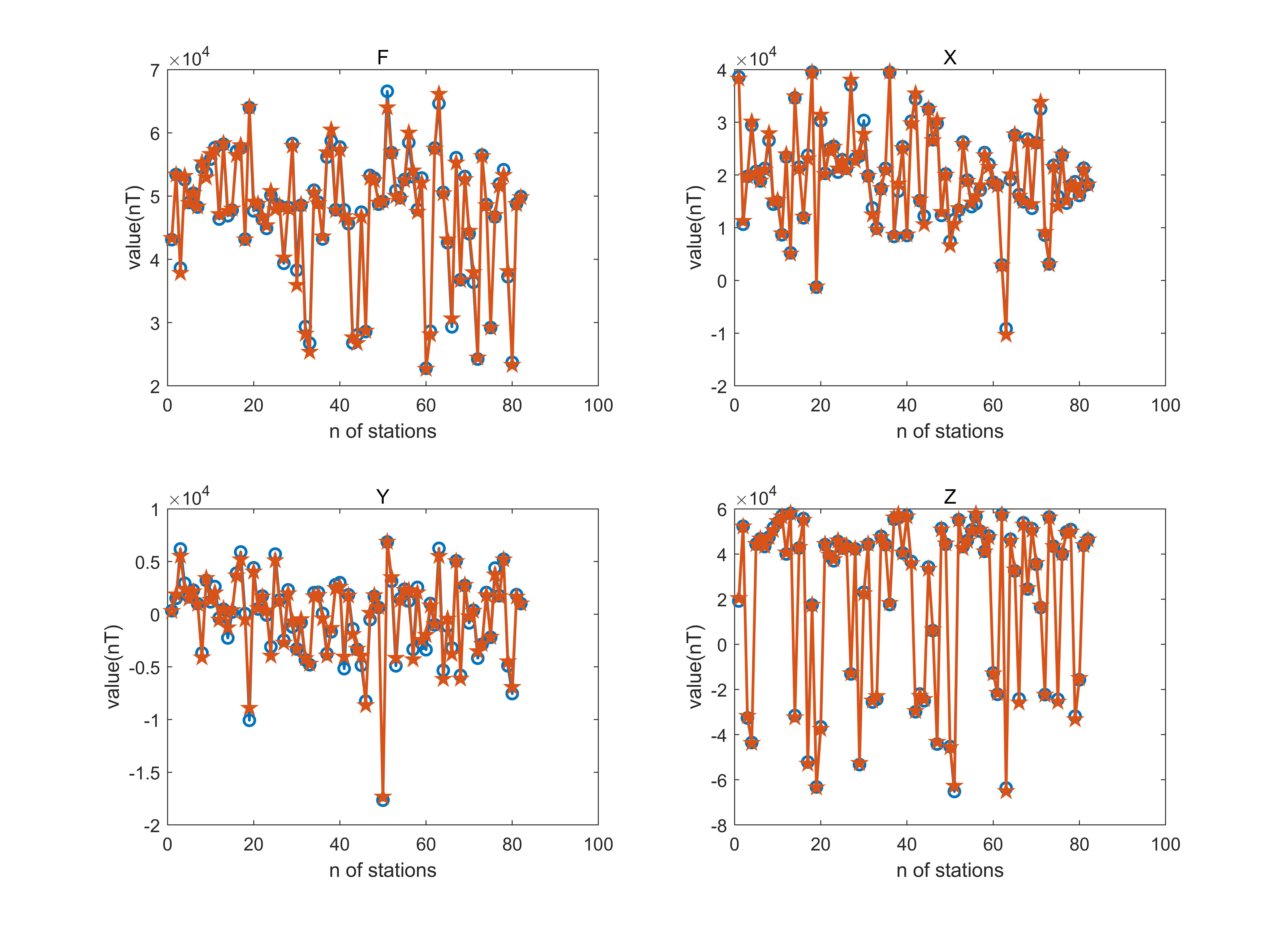
In order to evaluate the fitting effect of the model on the data, the prediction data on the original observation point were obtained by using $\mathbf{E} = \mathbf{A}\mathbf{m}$, and the error between the observation value and the prediction value was calculated, as shown in Figure 2, 3:
Global model from inverse Gauss Coefficient
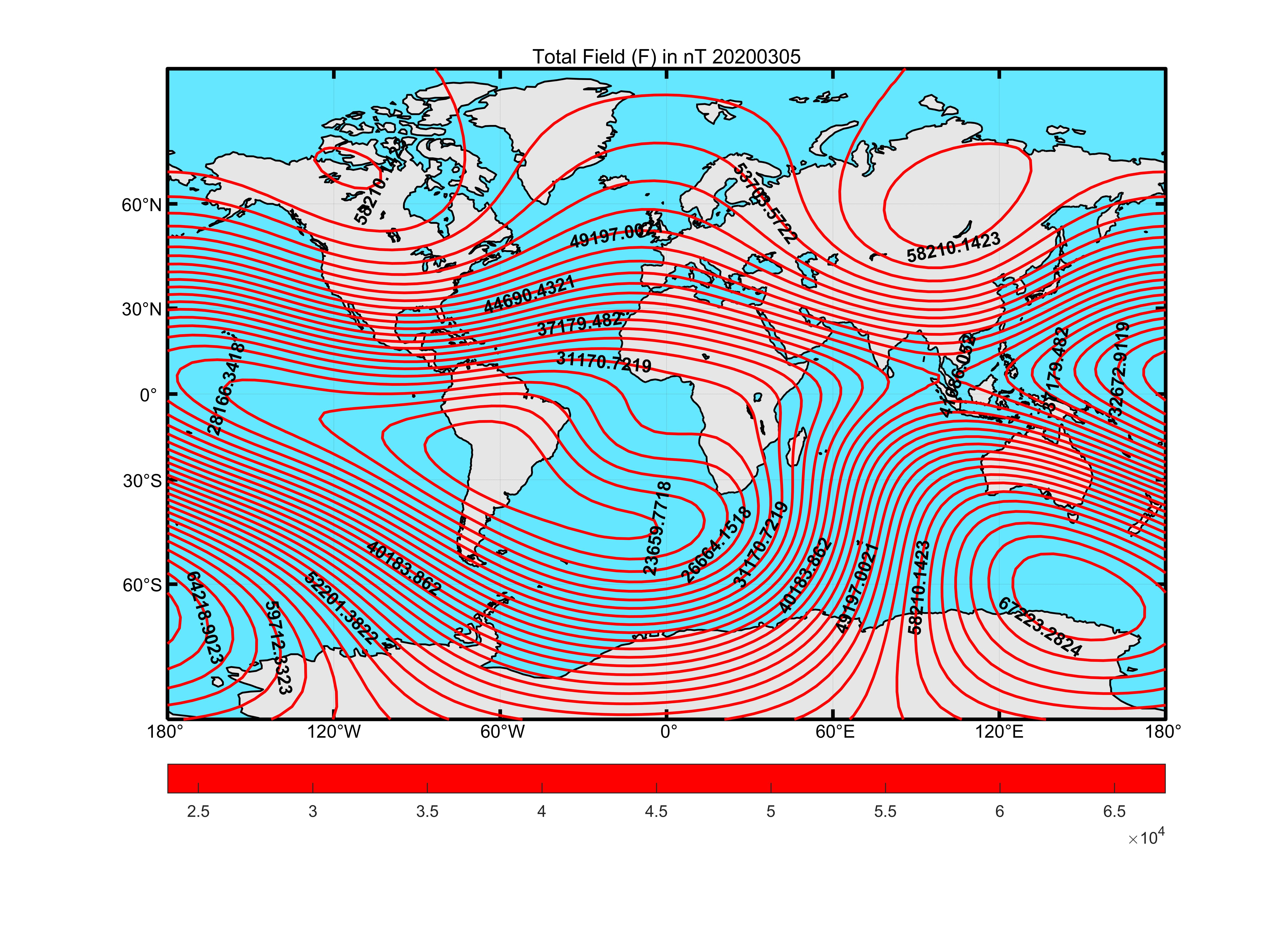
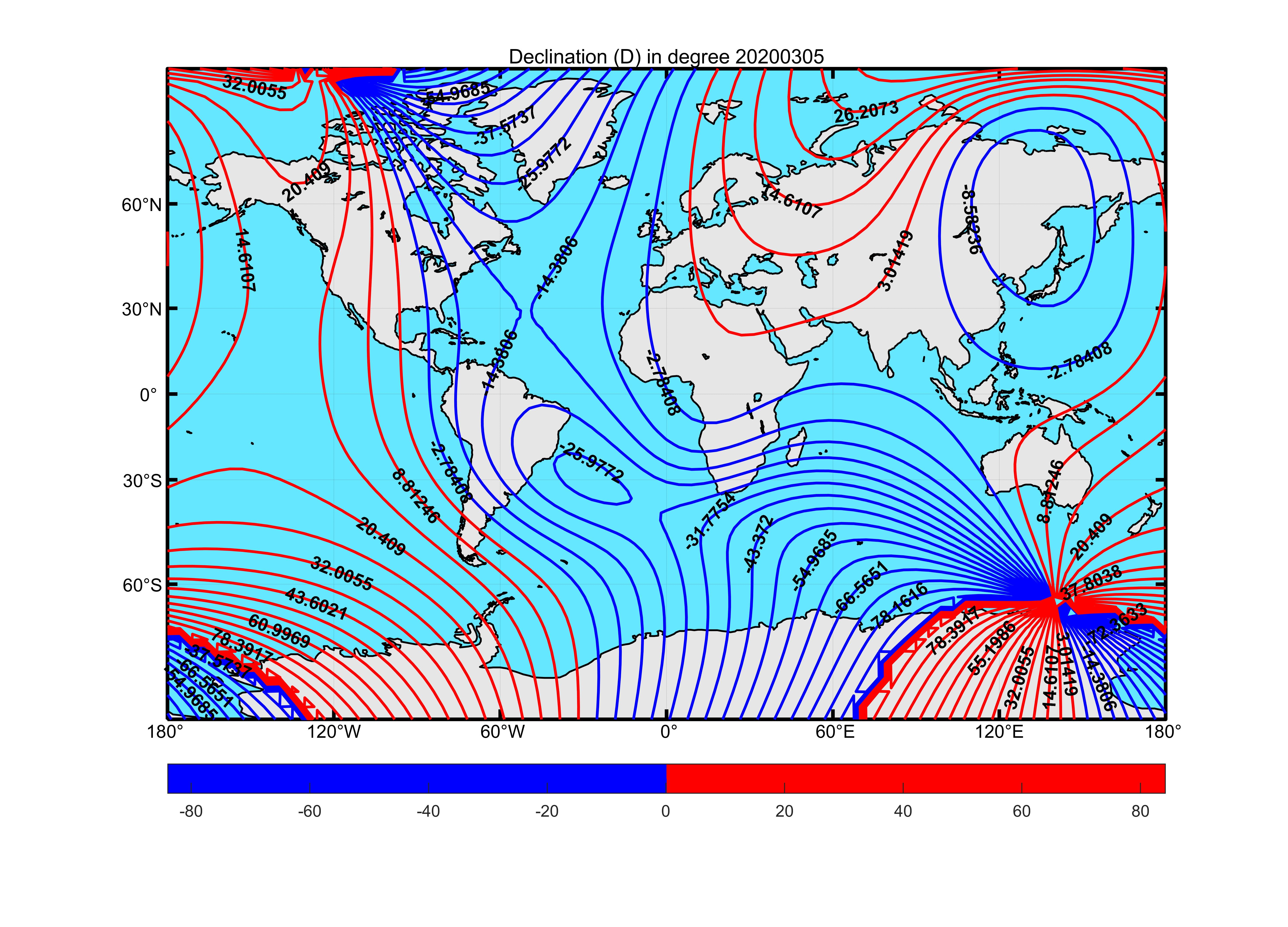
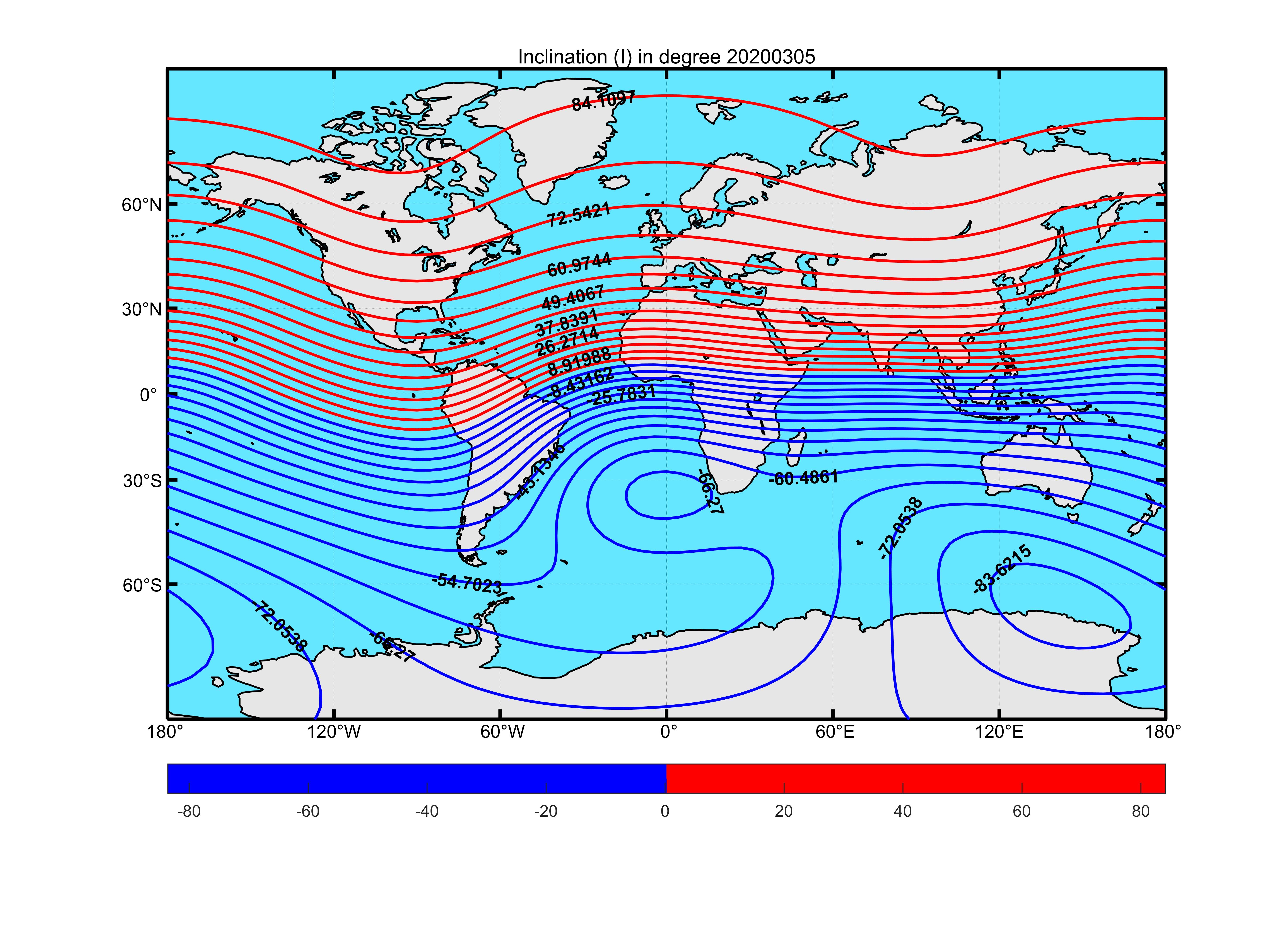
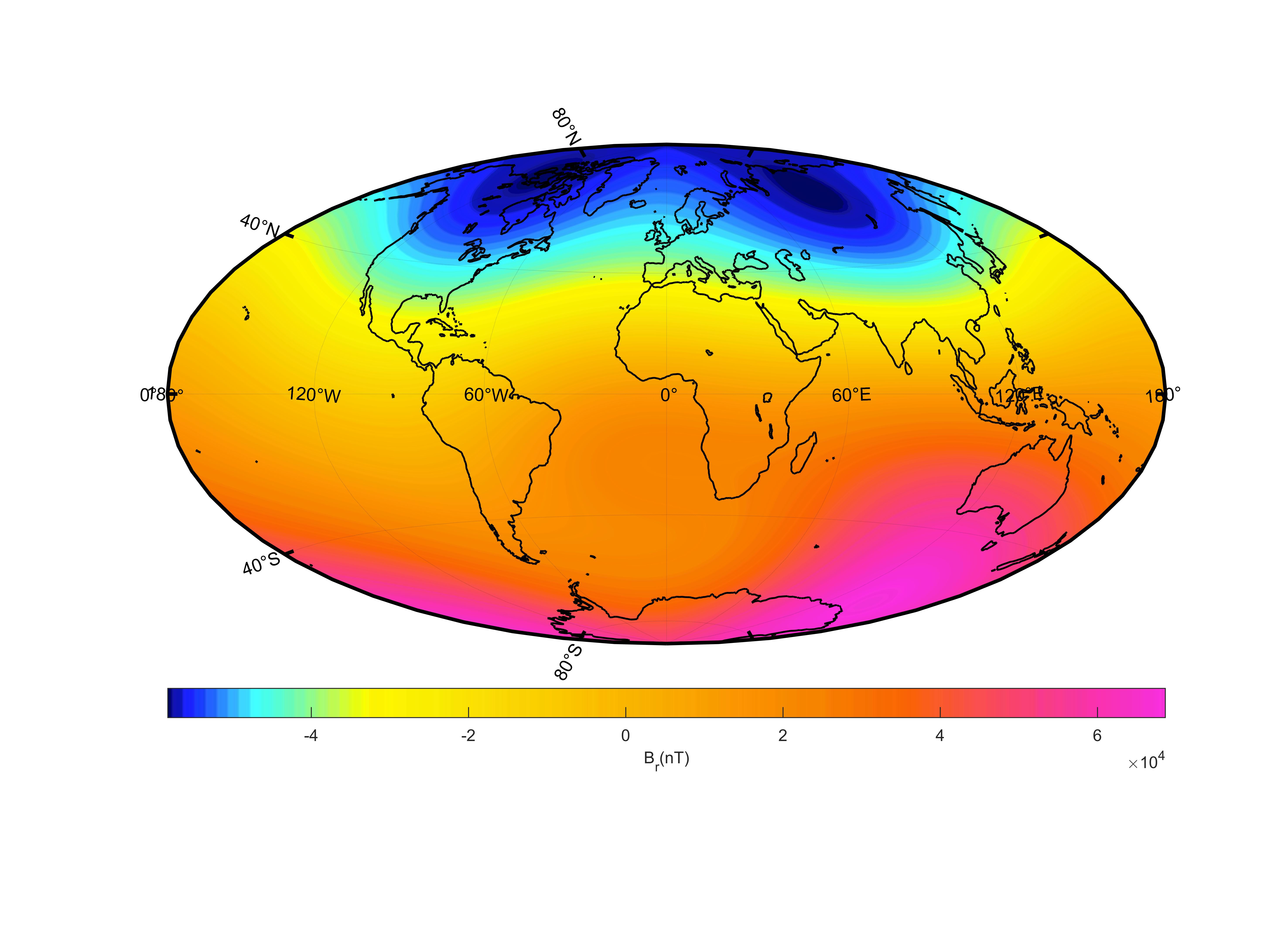
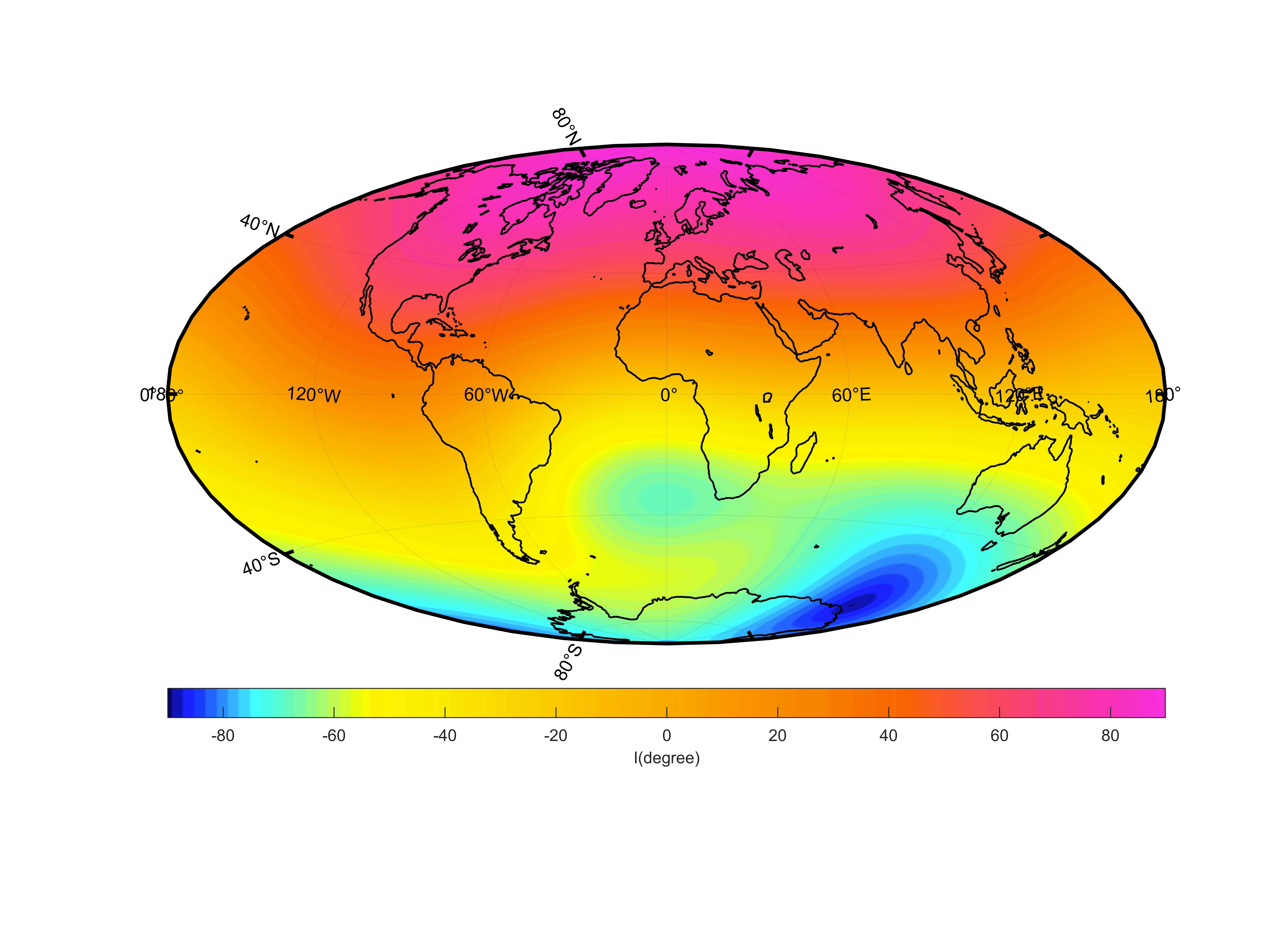
The inverse Gauss coefficient can be used to calculate the global magnetic field distribution, which has been shown in Figure 4-11
It is obvious that the South Atlantic magnetic anomaly is consistent with the known characteristics of the geomagnetic field, indicating that our model can reflect the characteristics of the geomagnetic field to a certain extent.
Comparison with IGRF-13
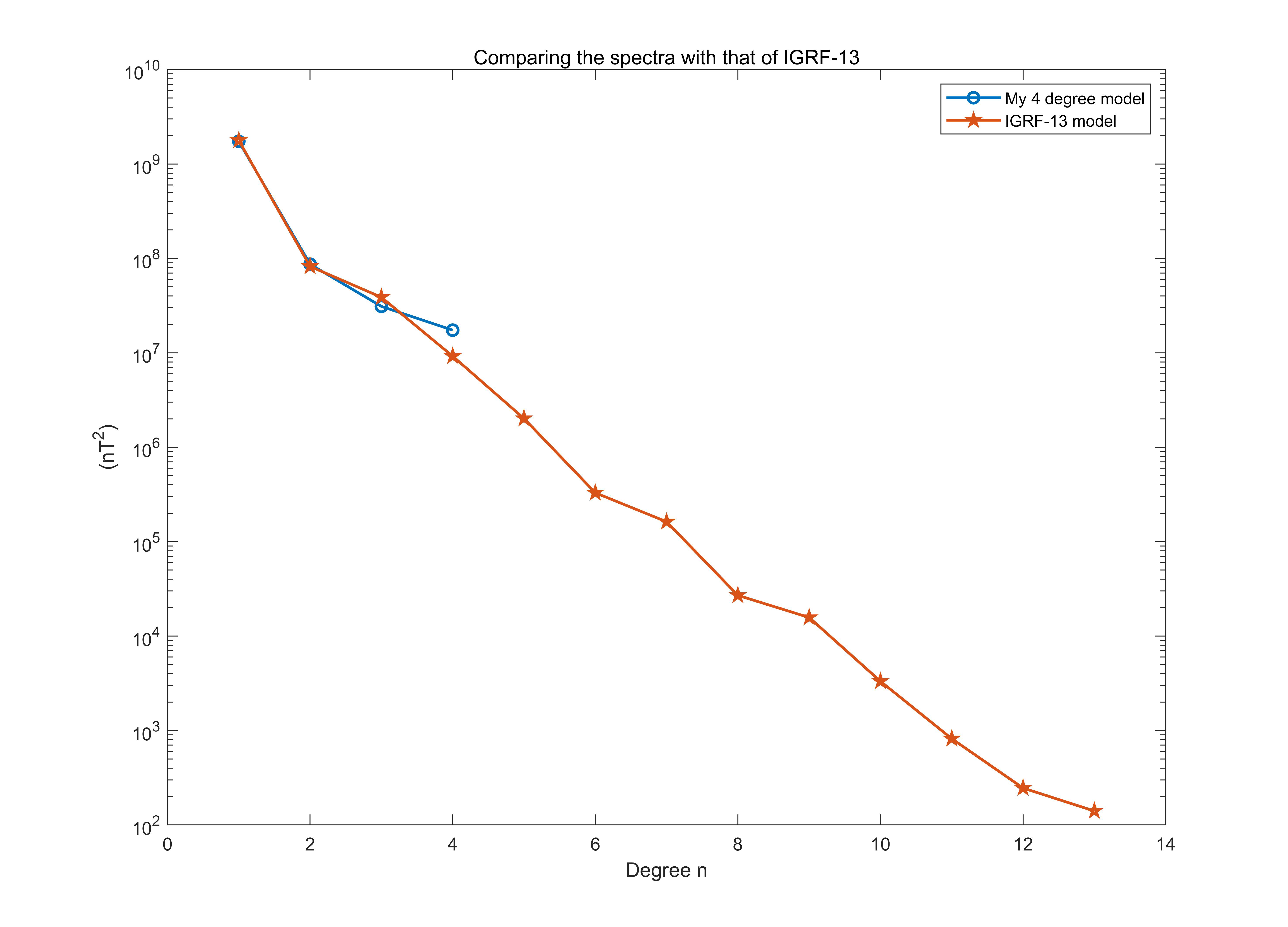
Compute the spectrum in SH degree by:
and compare them with the results of IGRF-13 (Figure 12) shown that the inversed Gauss coefficients are in good agreement with IGRF-13 model. The characteristics of the main earth’s magnetic field are almost the same, except for a small deviation when the degree is high.
Discussion
Through the inversion of the observed data, I got 24 Gauss coefficients, and used them to establish the global magnetic field model, draw the magnetic field distribution on the surface of earth. Compared with the IGRF-13 model, it has good consistency, but there are still subtle differences. The reason is that when we sift through the data, the distribution of observation stations is not well-distributed enough, and we can not achieve uniform distribution on a global scale. Therefore, the inversed model is greatly affected by the local data, even if we increase the degree of the spherical harmonic coefficient will not help, there will be even greater difference. If our model is to be more accurate, it will need to include satellite data that can orbit the Earth around, which will also take into account the effects of external fields on the geomagnetic field, making the model more accurate.
Code
The code can be attained at my github repository
Reference
[1] 聂琳娟, 许智铭. 利用SWARM星群磁测数据反演地球主磁场模型WHU-MM01[J]. 测绘地理信息, 2020, 45(05): 16–19.
[2] 徐文耀, 区加明, 杜爱民. 地磁场全球建模和局域建模[J]. 地球物理学进展, 地球物理学进展, 2011, 26(2): 398–415.
[3] Monika Korte, Catherine Constable. Continuous global geomagnetic field models for the past 3000 years[J]. Physics of the Earth and Planetary Interiors, 2003, 140(1): 73–89.
[4] N. W. Peddie. USGS model coefficients for continental U.S. and Hawaii (1985)[J]. Planetary and Space Science, 1992, 40(4): 561.
[5] An Homage to Gauss and His Model of the Earth’s Magnetic Field[J]. CMS Notes, .
[6] Davis J. Mathematical Modeling of Earth’s Magnetic Field[J]. .
[7] 白春华, 徐文耀, 康国发. 地球主磁场模型[J]. 地球物理学进展, 2008(4): 1045–1057.
[8] 冯春. Matlab实现IGRF国际地磁参考场模型的计算[J]. 内蒙古石油化工, 2014, 40(12): 43–46.
[9] 安振昌. 地磁场区域模型与全球模型的比较和讨论[J]. 物探与化探, 1991(04): 248–254.
[10] 刘元元, 王仕成, 张金生, 等. 最新国际地磁参考场模型IGRF11研究[J]. 地震学报, 2013, 35(1): 125-131+133-134+138.
[11] International Geomagnetic Reference Field (IGRF-13)[EB/OL]. /2022-05-28. https://wdc.kugi.kyoto-u.ac.jp/igrf/index.html.
[12] Alken P, Thébault E, Beggan C D, 等. International Geomagnetic Reference Field: the thirteenth generation[J]. Earth, Planets and Space, 2021, 73(1): 49.
[13] Finlay C C, Kloss C, Olsen N, 等. The CHAOS-7 geomagnetic field model and observed changes in the South Atlantic Anomaly[J]. Earth, Planets and Space, 2020, 72(1): 156.


